Logs with rhythm

By: John Vereen

            Looking at the graphs of y=log(x) and y=ln(x), it appears that these functions are related to exponentials. These are, indeed, related to exponential functions, but how? Unless specified otherwise, the function y=log(x) has a base of ten, so it is understood that we are actually writing y=log₁₀(x). But, what does this expression actually mean? In common Algebraic terms, it means that 10^y=x. So, the input of the log function is some number, and the function takes that number and makes it an exponent in a base 10 number system for the output. Similarly, we can think of the natural log function algebraically as e^y=x. This function takes the input and turns it into an exponent in a base e number system (e being the infinite sum (1/0! + 1/1!+ 1/2!...)).

            Let’s take a closer look at the structure of logarithmic functions and exponential functions and see just how the two are related. Let’s take the functions 10^x=y. If we were to input the value 2, we would obtain an output of 100. Now, Lets take the output of the exponential function, 100, and make it the input of the logarithmic function. We see that with an input of 100 for the logarithmic function, we get an output of 2! This is the case with all real numbers, which shows that these two functions have an inverse relationship.

            Now, let’s examine the graphs of some logarithmic functions.

Below, we have the graphs of y= log(x) and y=ln(x).

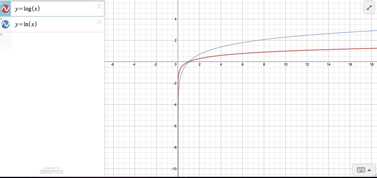
            Since we know that logarithmic functions are the inverse of exponential functions, we can also think about these graphs in the exponential form 10^y=x and e^y=x . We notice that each graph has a y value of 1 at the respective points x=10 and x=e. This tells us that ln(e)=1 and that log(10)=1, and that 10 and e must be the bases of each function. We know this because any number raised to a power of one gives us that exact same number. Another important fact about logarithmic funcitons is that, like exponential functions, they increase to infinity even though they appear to have an asymptote.

            With a(ln(x)) ; ln(bx) and a(log(x)) ; log(bx), we see some distinctions between each pair of graphs. After looking at these functions, I made some interesting observations. First of all, we notice that when a=b=1, then the graphs are identical for each respective ln and log function.

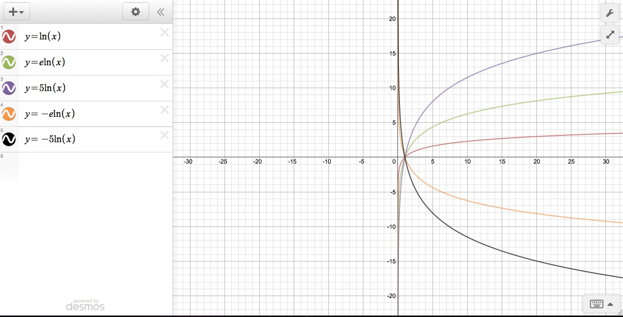
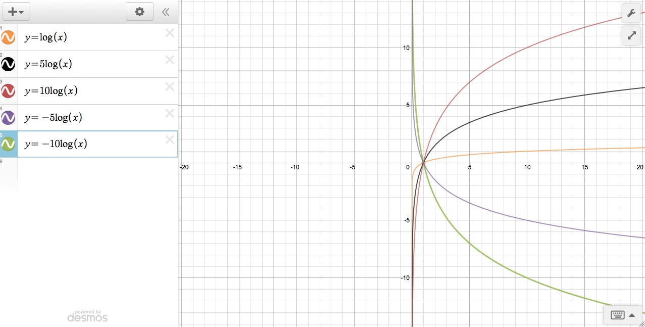
               There are many similarities factor a in y=a(log(x)) and y=a(ln(x)).  First of all, every graph of this form intersects at the point (1,0) because anything raised to the zero power is one. Before we further discuss the features of the graphs, let’s talk about how we can think about this variable a. An interesting characteristic of log and natural log functions is the “power rule.” The rule states that log_b (x^a) = a log_b (x). So basically, an exponent or “power” input a within the logarithm function is reduced to a multiplicative constant that scales the logarithm function.

               We see that positive inputs increase the scale of the a(log(x)) and  a(ln(x)) graphs , and they affect the magnitude of increase; the larger the number for a, the larger the magnitude by which that function increases. Also, we see that positive inputs for a produce standard a(log(x)) and  a(ln(x)) graphs that are increasing from (0,infinity) and are concave down. However, we see that negative inputs for a have the exact opposite affect on graphs of this form. These negative inputs cause the a(log(x)) and  a(ln(x)) graphs to be concave up and decreasing from (0,infinity). They are similar in the fact that the larger the number for a, the larger the magnitude by which that function decreases.

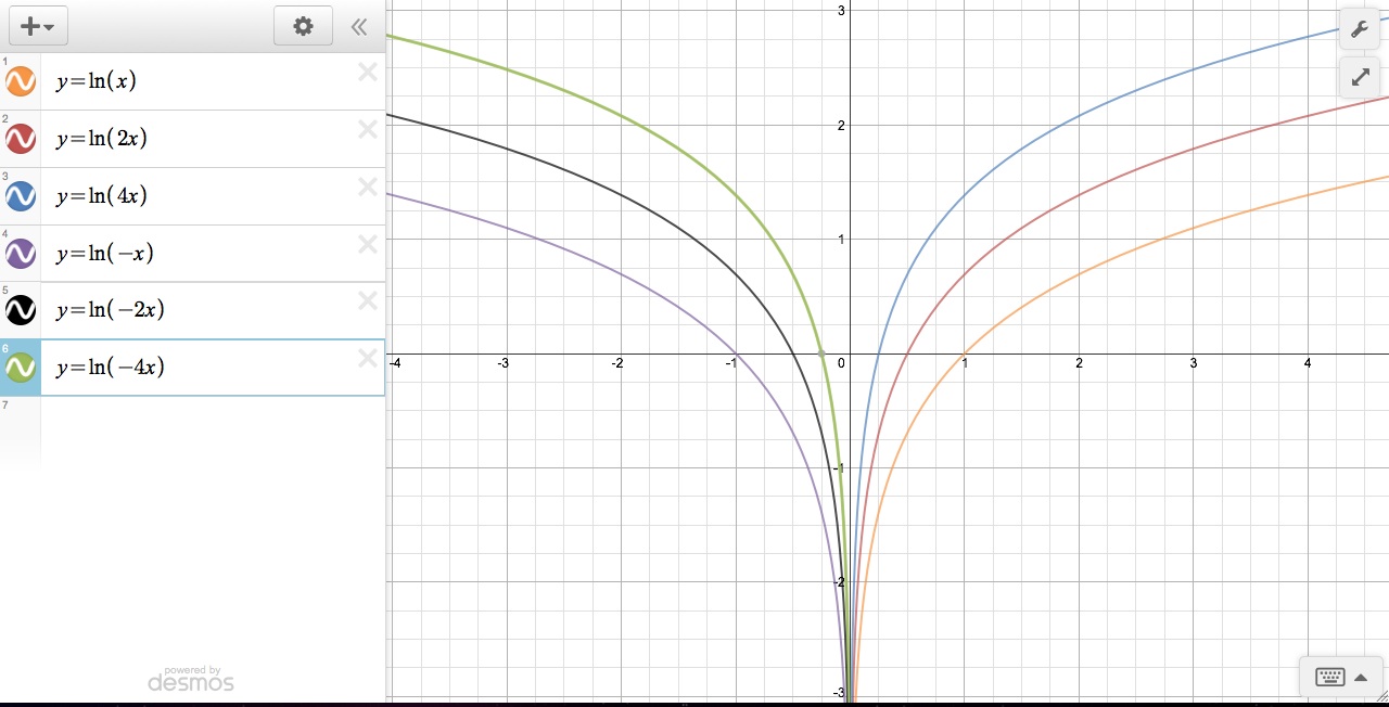
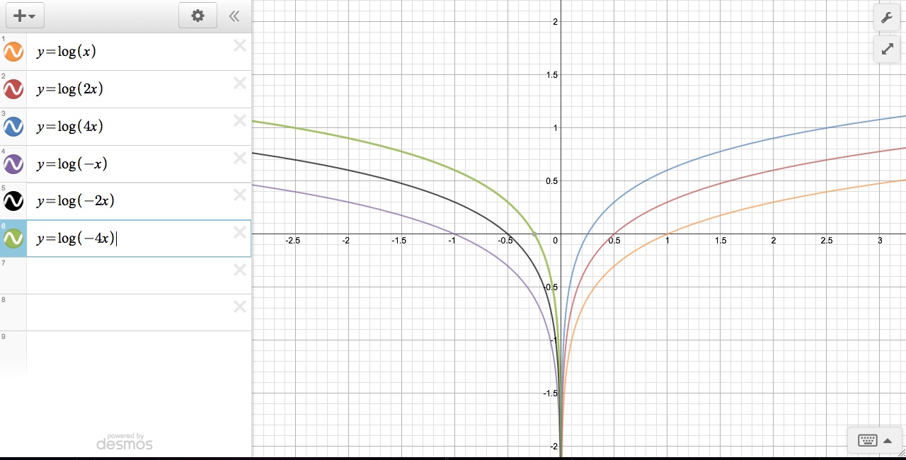
               We see many similarities with the factor b in y=(log(bx)) and y=(ln(bx)) (do not confuse b with base, it is a constant). A good look at each graph gives us the impression that b has the same effect on both functions. A great way to understand how b affects the graphs of the logarithmic functions is to see the meaning of the log and ln functions in exponential form. We can write these as 10^y=bx and e^y=bx or 10^y/b=x and e^y/b=x.

               This explains why each graph does not have a common intersection point of (1,0) like the y=a(log(x)) and y=a(ln(x)) graphs.  Yes, any number raised to the zero power is one. But, as we see in the equations 10^y/b=x and e^y/b=x, the constant b affects where the logarithmic function will intersect the x-axis or y=0. The larger the constant b, the closer to the origin the logarithmic graph will intersect the x-axis. Also, a larger constant b creates a taller logarithmic graph.

               We see a similar relationship when the constant b is negative. As a matter of fact, if one were to reflect a graph of the form y=(log(bx)) over the y-axis, then you would see the graph y=(log(-bx)) for any non-zero b. Negative a inputs affected the logarithmic graphs by changing the concavity. Also, the negative a constant kept the domain but changed the range. The negative b constant had the exact opposite effect on the logarithmic graphs. Negative b inputs maintained the concavity. However, the negative a constant maintained the range but changed the domain to (0, negative infinity).